Demographic Characteristics and Number of Extramarital Affairs
| ✅ Paper Type: Free Essay | ✅ Subject: Statistics |
| ✅ Wordcount: 7465 words | ✅ Published: 18 May 2020 |
Abstract
In this report, the relationship between the demographic characteristics of the individual and the number of extramarital affairs a person had in one year is discussed. The classical Poisson, quasi-Poisson, negative binomial regression models for count data, which belong to the family of generalised linear models, are introduced and applied to the “Affairs” dataset. Incorporating the over-dispersion and excess zeros problems, hurdle and zero-inflated regression models is also considered for modelling. Stepwise regression is used as a strategy for selecting variables. Moreover, the results of estimating the coefficients for the model are compared to find the model, which can fit the “Affairs” data best. As the measurement scales discussed in the report, it is better to treat the response variable “affairs” as ordinal data rather than count data. Hence, ordinal logistic regression is applied to the dataset in the advanced chapter.
Keywords: GLM, Poisson model, negative binomial model, hurdle model, zero-inflated model, ordinal logistic regression, stepwise regression.
1. Introduction
Although there are so many articles about extramarital affairs published in the popular press and media, scientific research on this sensitive topic developed slowly (Glass et al., 2004). In a previous study, evaluating the psychobiological correlates of extramarital affairs, Fisher et al. found that when compared with men without extramarital affairs, a higher androgenisation is present in men with infidelity (Fisher et al., 2009). Moreover, unfaithful subjects showed a higher risk of conflicts within the original family and higher stress at work (Bandini et al., 2010). As extramarital affairs seem to be an alpha-male activity (Fisher, 2012), most of researches paid more attention to males than females. However, marital infidelity is not only about males. So the purpose of this report is to test if there is a relationship between the demographic characteristics (include gender) and the number of having extramarital affairs. And then, choose a model that can fit the data best. There are 601 observations on 9 variables for the study, and the data are available from the magazine surveys leading by Psychology Today and Redbook in 1969 and 1974 (Fair, 1978).
The extent of having extramarital affairs is by no means small. In the two surveys used in this study,
men and
women had had at least one extramarital relationship during the year of the study (Fair, 1978). Therefore, some generalised linear models will be fitted with the variable “affairs” as response and the other eight variables as explanatory variables. Furthermore, variable selection and model comparison are implemented to find the best models for this problem. Besides, incorporating the measurement of scales (details in Chapter 2), the outcome variable “affairs” is treated as count data in Chapter 4, and it is treated as ordinal data in Chapter 5. As a result, the purpose of the count data regression in this report is inference, and the purpose of ordinal logistic regression is prediction.
The structure of the project is as follows. Chapter 2 describe the data and Chapter 3 introduced the methods. Chapter 4 contains a standard analysis of count data regression models: explanatory analysis, model verification, model comparison and model selection. Chapter 5 includes ordinal logistic regression and summary of conclusions, discussion of limitations and the further task is discussed in Chapter 6.
2 The Data
This project uses data from Fair (1978). The data are gathered from two magazine questionnaires on sex in the 1960s and 1970s. Psychology Today (PT) conducted the first survey in 1969, and the second survey was conducted in 1974 by Redbook (RB). The questionnaires included the question about the number of extramarital affairs a person had in one year as well as some questions about other aspects of sexual behaviour. That is, various demographic and economic characteristics of the individual (Fair, 1978).
As the methods of statistical analysis depend on the measurement scales of the response (Dobson, Annette J; Barnett, Adrian G, 2008), the measurement scales of variables need to be discussed first. The four fundamental levels of measurement scales (nominal, ordinal, interval and Ratio) provided by Entry (Entry, 1990) are used in this report. The definitions are given below:
- Nominal scale: a scale used for labelling variables into different categories and does not involve a quantitative value or order.
-
Ordinal scale: a scale used when there is some natural order or ranking between the categories. For example: diastolic blood pressures groups as
- Interval scale: a scale used when rank-ordered data categories may be placed equidistantly on a scale with an arbitrary zero point. Besides, the difference between any two values is meaningful.
- Ratio scale: a scale used when equidistant rank-ordered data categories may be placed on a scale with an absolute zero point.
Nominal and ordinal data are categorical variables as well as interval and ratio scale are continuous variable (Dobson, Annette J; Barnett, Adrian G, 2008). Table 1 shows the data description for the “Affairs” dataset.
From the table, it is clear that all predictor variables in the dataset are categorical variable. Besides, it is better to treat the response variable “affairs” as an ordinal categorical variable rather than a count variable. Since the value recorded for the response variable “affairs” (
) is not always the real number of times of having affairs. For example, when
, it means that the observation cheated every month, every week, or even every day. However, the topic of the dissertation belongs to the theme “Count data regression models”, so the response variable “affairs” is treated as count data in Chapter 4 (Standard analysis of the data) and as an ordinal variable in Chapter 5 (Advanced chapter).
Table 1 Data description
|
Variable Name |
Notation |
Description of Variable |
Values of Variable |
Scale |
|
|
|
How often engaged in extramarital affairs during the past year? |
0 = none, 1 = once, 2 = twice, 3 = 3 times, 7 = 4-10 times, 12 = monthly/weekly/daily |
Ordinal |
|
|
|
Gender |
0 = female, 1 = male |
Nominal |
|
|
|
Age |
17.5 = under 20, 22 = 20–24, 27 = 25–29, 32 = 30–34, 37 = 35–39, 42 = 40–44, 47 = 45–49, 52 = 50–54, 57 = 55 or over |
Ordinal |
|
|
|
No. of years married |
0.125 = 3 months or less, 0.417 = 4–6 months, 0.75 = 6 months-1 year, 1.5 = 1–2 years, 4 = 3–5 years, 7 = 6–8 years, 10 = 9–11 years, 15 = 12 or more years. |
Ordinal |
|
|
|
Are there children in the marriage? |
0 = no, 1 = yes |
Nominal |
|
|
|
How religious |
1 = anti, 2 = not at all, 3 = slightly, 4 = somewhat, 5 = very |
Ordinal |
|
|
|
Level of education |
9 = grade school, 12 = high school graduate, 14 = some college, 16 = college graduate, 17 = some graduate work, 18 = master’s degree, 20 = Ph.D. |
Ordinal |
|
|
|
Occupation |
1– 7, according to Hollingshead classification (reverse numbering) |
Ordinal |
|
|
|
How rate marriage |
1 = very unhappy, 2 = somewhat unhappy, 3 = average, 4 = happier than average, 5 = very happy |
Ordinal |
3. Description of the methods
In this section, the theory and its implementation in R for some basic count data regression models and their zero-augmented extensions are described (see Table 2 for an overview). In addition, the other methods used in this report are also showed in this Chapter.
The Poisson, negative binomial models and ordinal regression model (OLR) are described in a generalized linear model (GLM) framework. The Poisson regression model is provided in R by the
function (Chambers JM, Hastie TJ, 1992) in the stats package. The
and
functions are in theMASS package, respectively (Venables WN, Ripley BD, 2002). Besides, rather than ordinary least squares (OLS), the methods above use maximum likelihood estimation (MLE) to estimate the parameters, which means that they are depended on large-sample approximations.
Poisson regression is often used for modelling count data. However, as count data sets sometimes show over-dispersion (or have a large number of zeros), the classical Poisson regression model for count data does not always fit the data well. To solve the over-dispersion problem, quasi-Poisson model and negative binomial (NB) regression model, which including additional shape parameter can be considered (Achim Zeileis, Christian Kleiber, Simon Jackman, 2008). Another two models, which can also solve these two problems, are hurdle and zero-inflated model. The hurdle and zero-inflated extensions of these models are provided by the functions
and
in package pscl (Jackman, 2008). The function
in package MASS can fit the model when the outcome variable is treated as an ordered factor. The table below summarised the models considered in this report. Further information about the models and relative code in R can be found in the respective references.
Table 2 Methods of statistical analysis considered in the report
|
Response |
Explanatory Variables |
Type |
Distribution |
Methods |
|
Count |
Categorical & Continuous |
generalized linear model |
Poisson |
Maximum Likelihood |
|
Negative Binomial (NB) |
Maximum Likelihood |
|||
|
zero-augmented |
Zero-inflated Poisson (ZIP) |
Maximum Likelihood |
||
|
Zero-inflated NB (ZINB) |
Maximum Likelihood |
|||
|
Ordinal |
Categorical & Continuous |
generalized linear model |
– |
Maximum Likelihood |
3.1 Generalised linear model (GLM)
Generalised linear regression is helpful in the social sciences and economics (Achim Zeileis, Christian Kleiber, Simon Jackman, 2008). In this section, the framework, assumptions and the main idea of generalised linear regression models (GLM) are shown.
3.1.1 Assumptions of GLM
-
The observations
are independently distributed.
-
The dependent variable
is from an exponential family (e.g. binomial, Poisson, multinomial, normal).
- A linear relationship between the transformed response (the link function) and the explanatory variables.
- The homogeneity of variance does NOT need to be satisfied.
- Errors need to be independent but NOT normally distributed.
(Hilbe, 2014)
3.1.2 Main ideas of generalised regression modelling
The primary motivation for the model is to figure out the relationships between the number of having affairs and other aspects of characteristics. The classical generalised regression modelling process, which is given by the book “An Introduction to Generalized Linear Models” (Dobson, Annette J; Barnett, Adrian G, 2008), involves four steps:

- Specifying three components to models:
- The linkage – an equation linking the outcome and explanatory variables.
-
Systematic Component – specifies the explanatory variables (
) in the model and creates linear predictor; e.g.,
.
-
Random Component – the probability distribution of outcome variable (
).
- Estimating parameters in the models.
- Checking how well the models fit the data.
- Making inferences: for example, testing hypotheses and calculating confidence intervals for parameters.
Since different statistical analysis methods have different linkage, and statistical analysis methods depend on the measurement scales of the response and explanatory variables. The next section summarised the model frame for the GLM models considered in this report.
3.1.3 Model frame
Generalised linear models (GLMs) are generalised from the linear models, which describe the dependence of a scalar variable
on a vector of
. The conditional distribution
of response variable belongs to the exponential family, which can be written as:
Where
is the natural parameter and the functions
and
are known from which member of the family is used (Achim Zeileis, Christian Kleiber, Simon Jackman, 2008).
For example, for the binomial and Poisson distribution,
, the conditional mean and variance of
are given below (Dobson, Annette J; Barnett, Adrian G, 2008):
The dependence of the conditional mean
can be described via
where
is link function and
is the vector of regression coefficients, which are estimated by maximum likelihood (ML) method (Chambers JM, Hastie TJ, 1992).
3.1.3.1 Treat the variable “affairs” as count data
Poisson model
The classical regression model used for modelling count data is the Poisson regression. The probability density function for the response
is:
which is of exponential family. Canonical link for Poisson model is
resulting in a log-linear relationship between mean of the response
and the linear predictors. Since the variance in the Poisson model is identical to the mean, over-dispersion, which means that the variance is bigger than the mean, may appear in practice (Hilbe, 2014). In R, Poisson model can be easily applied in the
call just by setting
.
Quasi-Poisson model
One way of modelling over-dispersed count data is using quasi-Poisson model, which means using the mean and the variance function from the Poisson GLM, but leaving the dispersion parameter unrestricted (Jay M. Ver Hoef, Peter L. Boveng, 2007). Such that
Where
. In the equation,
is an over-dispersion parameter which can be estimated from the data. In R, the quasi-Poisson model can be fitted with the
function, by simply setting
.
Negative binomial models
Another formal way of dealing with over-dispersion is to assume a negative binomial (NB) distribution for
, which can be regarded as a gamma mixture of Poisson distributions. The probability density function of NB models can be written as:
Where
is the mean,
is a shape parameter and
is the gamma function. For every
, this fits equation (1) and thus is another particular case of the GLM framework (Jay M. Ver Hoef, Peter L. Boveng, 2007). In R, the coefficient
can be calculated using the function
from the package
.
3.1.3.2 Treat the variable “affairs” as ordinal data
If there is an apparent natural order among the response categories, then ordinal logistic regression models can be considered. Suppose
is an ordinal outcome with
categories. Then
is the cumulative probability of
less than or equal to the
th category
. It is clear that
. The log odds (or the
) of being less than or equal
th category is defined as
for
.
Due to the parallel lines assumption in R system (which means that the intercepts are different for each category but the slopes are the same among categories), the ordinal logistic regression models have the following general form:
for
(McCullagh, 1980).
In R, the coefficient
can be calculated using the function
, and the ordinal logistic regression model is parameterized as
Where
and p is the number of
.
in R is a kind of proportional odds logistic regression models, with proportional odds assumption. And to have the model return the Hessian which is used to get standard errors,
is specified.
3.2 zero-augmented model
In addition to over-dispersion, many count data sets have more zero observations than allowed for the Poisson model. Two kinds of models that can solve both of the problems are Hurdle models and zero-inflated models (Lambert D, 1992).
The density of the zero-inflated is a mixture of a point mass at zero
and a count distribution
. The probability of observing a zero count is
Hence, the probability density function of zero-inflated models can be written as:
where
is the indicator function and the corresponding equation for the mean is
using the canonical log link (Achim Zeileis, Christian Kleiber, Simon Jackman, 2008). In R, zero-inflated count data models can be fitted with the
function from the
package.
The hurdle model combines two-component models: a hurdle component models zero vs. larger counts and a truncated count component, such as Poisson or negative binomial, which is employed for positive counts (Achim Zeileis, Christian Kleiber, Simon Jackman, 2008).
That is, the hurdle model combines a zero hurdle model
(right-censored at y = 1) and a count data model
(that is left-truncated at y = 1):
The model parameters
, and potentially one or two additional dispersion parameters
(if
or
or both are negative binomial densities) are estimated by maximum likelihood. The corresponding mean regression relationship is given by:
again the canonical log link is used. In R, hurdle count data models can be fitted with the
function from the pscl package (Jackman, 2008).
3.3 Stepwise regression
In statistics, there are many different strategies for selecting variables for a regression model. The usual method to choose a model is (backward/ forward) stepwise. “Backward stepwise” is used in this report, and the details are described below (Vincent Calcagno, Claire de Mazancourt, 2010).
- Fit the full model first and find out the terms that are not statistically significant, that is, whose removal does not signicantly reduce the fit of the model.
- Removes the least-significant one, thus obtaining a new “simplified” model.
- Repeat the procedure until all effects in the formula are found significant.
Besides, several methods that can determine whether the removal of a given term at each test is significant (Venables WN, Ripley BD, 1997).
- Hypothesis test tools, such as the chi-square test, or likelihood ratio (LR) test, involve specifying a significance threshold for the p values (e.g., 5%).
- Information criteria (IC), e.g., the Akaike information criterion (AIC).
Choosing model by AIC in a stepwise algorithm is convenient, and the choice of predictor variables can be carried out by an automatic procedure in R via
CITATION Dob08 l 2057 (Dobson, Annette J; Barnett, Adrian G, 2008).
There are three directions for
function to select the model – “both”, “backward”, or “forward”. The only fundamental difference between backward and forward stepwise selection is whether there is the explanatory variables in the model at first (Hilbe, 2014):
- without predictors (forward);
- with all the predictors (backward).
As in GLM, the deviance is not simply related to the maximised log-likelihood (Achim Zeileis, Christian Kleiber, Simon Jackman, 2008). There is a potential problem when using the stepwise algorithm in GLM. Nevertheless, the Poisson and Binomial families have fixed scale by default (Hilbe, 2014), so it is not necessary to amend it in this case.
3.4 The variance inflation factor (VIF)
Multicollinearity occurs when there are high correlations among predictor variables, leading to unreliable and unstable estimates of regression coefficients (Allison, 2012). In this report, the variance inflation factor (VIF) is used to diagnose the multicollinearity. The VIF can be calculated by fitting a linear regression of that predictor on all the other predictors, and then the
can be obtained from the regression. The VIF is just
. It can be accomplished via
in R. Moreover, for VIF in R, if the degree of freedom for any predictors in an unweighted linear model is bigger than 1, then generalised variance-inflation factors (Fox, J; Monette, G, 1992) are calculated.
Though the interpretations for GVIF is different, the rule of
(Philipp, 2019) is used in some publications, which would equal to
a VIF of 4 for one-coefficient variables. The same criterion used in this report. That is, if
, multicollinearity appears at a high rate.
3.4 Over-dispersion Test
The function
can be found in the package AER in R, which implements a test for over-dispersion by Cameron and Trivedi (Cameron; Trivedi, 1990).
As in a Poisson model, the mean
and the variance
are the same, the over-dispersion test sets
, where the constant
means under-dispersion and
means over-dispersion. The function
is the monotone function (linear is the default). The test statistic used is a
statistic which is asymptotically standard normal under the null.
If the p-value in the output is smaller than 0.05, then the null hypothesis will be rejected. That is, there is enough evidence of over-dispersion.
4 Standard analysis of the data
In this section, the variable “affairs” is treated as a count variable; the relative models mentioned in the previous section are applied to the “Affairs”. Before the models are fitted, fundamental exploratory analysis of the dataset is carried out. At the end of the chapter, fitted models discussed in this chapter are compared. As the mean functions for the models are similar but the fitted likelihoods are different, the models’ performance differently when solving over-dispersion and/or the number of zero counts problems.
4.1 Exploratory data analysis
As there are no missing values in the dataset, the first step of exploratory data analysis is to obtain a first overview of the response variable. A histogram of the frequency of extramarital sex is carried out below. Since the values of the variable “affairs” are not always the real frequency, argument
is used to re-label the frequency.
The figure below shows both substantial variation and a rather large number of zeros (see Figure 1). Besides, the second step in the exploratory analysis is always to look at the partial relationships, which can be shown by pairwise bivariate displays of the response variable against each of the predictor variables. Only the plot for the number of having affairs against age group is shown in this report, and the code for analogous displayed can be found in the R code section.
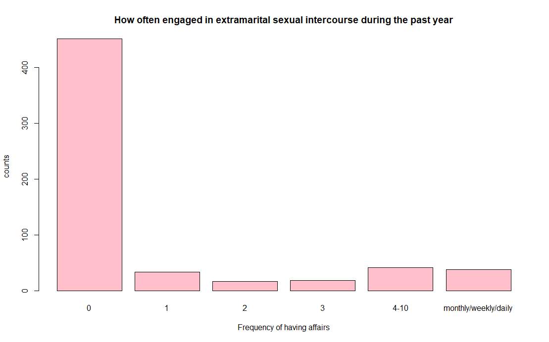
Figure 1 How often engaged in extramarital sexual intercourse during one year
Simple scatterplot is not useful as variables are ordinal categorical variables producing overlap. Boxplot or bar plot can overcome the problem of overlap, but as there are a large number of outliers in the dataset, the bar plot performance better. Besides, the numbers of observations for each group are different,
is used instead of
to eliminate the population effects. Figure 2 shows the bar plot of the number of having affairs against age group.
All displays show that the number of having affairs increases or decreases with the independent variables as expected. For example, the bar plot in Figure 2 shows that both the probability of having affairs and the frequency of cheating are higher when people at their middle age or when they are rather young, which fits the common sense.
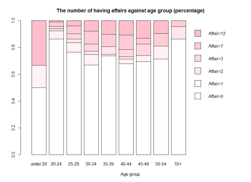
Figure 2 The number of having affairs against years of married (percentage)
As multicollinearity is a common problem when estimating linear or generalised linear models, the most widely used diagnostic for multicollinearity – generalised variance-inflation factors (GVIF) – is used in the report (the details are in Section 3.4). Table 3 shows the degree of freedom and the (generalised) variance inflation factor (GVIF) for each predictor.
Table 3 GVIF for the predictors
|
|
GVIF |
Df |
|
|
|
factor(gender) |
1.692950 |
1 |
1.301134 |
Yes |
|
factor(age) |
9.409511 |
8 |
1.150398 |
Yes |
|
factor(yearsmarried) |
10.171756 |
7 |
1.180203 |
Yes |
|
children |
1.923983 |
1 |
1.387077 |
Yes |
|
factor(religiousness) |
1.354615 |
4 |
1.038669 |
Yes |
|
factor(education) |
3.249556 |
6 |
1.103194 |
Yes |
|
factor(occupation) |
3.132359 |
6 |
1.099823 |
Yes |
|
factor(rating) |
1.485101 |
4 |
1.050678 |
Yes |
From the table, Multicollinearity could be ignored safely in this case.
4.2 Poisson regression
As a first attempt to capture the relationship between the number of having extramarital affairs and all predictor variables, the basic Poisson regression model is used. The backward stepwise regression procedure identified the model which included 8 predictors “gender”, “age”, “yearsmarried”, “children “, “religiousness”, “education”, “occupation” and “rating”, as the one which produced the lowest value of AIC.
Significant coefficients are expected after the stepwise regression procedure, but it is not true in the case. Most coefficients are highly significant except coefficients for “gender” and “children”. Here are some reasons: the stepwise regression procedure in R selects the model based on Akaike Information Criteria (AIC), not p-values. The purpose is to find the model with the smallest AIC by removing or adding variables. Since each variable in the model is a categorical variable, this leads to likelihood-ratio tests allow higher p-values when selecting the models (Achim Zeileis, Christian Kleiber, Simon Jackman, 2008). Since the coefficients for “gender” and “children” are not significant, they are deleted one by one via deleting the variable with the biggest p-value in Chi-square tests.
Also, the test of over-dispersion mentioned in Chapter 3 is used, and there is evidence of over-dispersion (
is estimated to be
, and the p-value is ) which reject the assumption of equidispersion (i.e.
). Therefore, it is more reasonable to explore other models to solve the over-dispersion (and excess zeros) problem. The values of coefficients are suppressed here and are presented in tabular form in Table 7.
4.3 Quasi-Poisson Model
As AIC is not defined for the quasi-Poisson model, the stepwise regression
in R cannot proceed, so choosing a model by the chi-square test in a stepwise algorithm is considered. As a result, the predictor “occupation”, “gender”, “children”, “education”, “yearsmarried” are deleted in order. As the estimated dispersion of
, which is larger than 1, confirming that over-dispersion is present in the data. Table 4 shows the deviances and AIC of Quasi-Poisson model.
Table 4
|
Null deviance: 2925.5 on 600 degrees of freedom |
|
Residual deviance: 2250.4 on 584 degrees of freedom |
|
AIC: NA |
From the table, the residual deviance for the Poisson model is
, which is very large compared with the
, indicating a poor fit if the Quasi-Poisson is the correct model for the response. That is, even if the over-dispersion is showed by the estimated dispersion of
, more models could be explored to find the most suitable model for the “Affairs” dataset. The values of coefficients are presented in Table 7.
4.4 negative binomial model
A more formal way to deal with over-dispersion in a count data regression model is to use a negative binomial model. As shown in Table 7, both the values of regression coefficients and significance of coefficients are somewhat similar to the quasi-Poisson. Thus, in terms of predicted means, the two models give very similar results. Table 5 shows the deviances and AIC of the negative binomial model.
Table 5
|
Null deviance: 408.73 on 600 degrees of freedom |
|
Residual deviance: 340.85 on 584 degrees of freedom |
|
AIC: 1479.2 |
From Table 5, the residual deviance for the Poisson model is
, which is relatively small compared with the
distribution, indicating a good fit if the negative binomial is the correct model for the response.
4.5 Zero-inflated regression & Hurdle regression
In this section, the zero-inflated regression model and the Hurdle regression model are applied to the “Affairs” dataset. The backward stepwise regression procedure identified the model which included four predictors “gender”, “age”, “religiousness” and “rating”, as the one which produced the lowest value of AIC. As the hurdle regression model and ZINB regression model are based on the same variables, the better model could be selected via likelihood. Table 6 shows the log-likelihood of the two models. From the table, the log-likelihoods are almost same, and zero-inflated model is a bit better than Hurdle model in this case. See Table 7 for a more concise summary.
Table 6
|
|
Log-likelihood |
|
Hurdle regression |
-683.4 on 37 Df |
|
Zero-inflated regression |
-683.1 on 37 Df |
4.6 Comparison of the models
Table 7 Summary of fitted count regression models for Affairs dataset
|
Type Distribution Object |
GLM Poisson Quasi-P NB
|
zero-augmented Hurdle-NB ZINB
Count Zero Count Zero |
|||||
|
(Intercept) |
2.145 |
3.668 |
3.805 |
2.742 |
2.776 |
2.748 |
-2.923 |
|
factor(gender)male |
– |
– |
– |
-0.334 |
0.279 |
-0.383 |
-0.407 |
|
factor(age)22 |
-2.308 |
-2.443 |
-2.512 |
-1.016 |
-2.306 |
-0.971 |
2.238 |
|
factor(age)27 |
-2.247 |
-1.834 |
-1.691 |
-0.662 |
-1.855 |
-0.641 |
1.837 |
|
factor(age)32 |
-2.183 |
-1.284 |
-1.271 |
-0.566 |
-1.291 |
-0.582 |
1.231 |
|
factor(age)37 |
-2.348 |
-1.236 |
-1.464 |
-0.045 |
-1.825 |
-0.002 |
1.959 |
|
factor(age)42 |
-2.278 |
-1.079 |
-1.271 |
-0.324 |
-1.423 |
-0.353 |
1.445 |
|
factor(age)47 |
-2.109 |
-0.886 |
-0.373 |
0.167 |
-1.194 |
0.238 |
1.341 |
|
factor(age)52 |
-2.177 |
-1.098 |
-0.448 |
0.066 |
-1.485 |
0.121 |
1.615 |
|
factor(age)57 |
-4.036 |
-2.775 |
-1.664 |
-0.511 |
-2.856 |
-0.368 |
2.948 |
|
factor(yearsmarried)0.417 |
-0.106 |
– |
– |
– |
– |
– |
– |
|
factor(yearsmarried)0.75 |
1.561 |
– |
– |
– |
– |
– |
– |
|
factor(yearsmarried)1.5 |
1.521 |
– |
– |
– |
– |
– |
– |
|
factor(yearsmarried)4 |
2.275 |
– |
– |
– |
– |
– |
– |
|
factor(yearsmarried)7 |
2.597 |
– |
– |
– |
– |
– |
– |
|
factor(yearsmarried)10 |
2.954 |
– |
– |
– |
– |
– |
– |
|
factor(yearsmarried)15 |
3.058 |
– |
– |
– |
– |
– |
– |
|
childrenyes |
– |
– |
– |
– |
– |
– |
– |
|
factor(religiousness)2 |
-0.791 |
-0.825 |
-0.715 |
0.012 |
-1.134 |
0.067 |
1.266 |
|
factor(religiousness)3 |
-0.658 |
-0.621 |
-0.612 |
-0.061 |
-0.675 |
0.006 |
0.792 |
|
factor(religiousness)4 |
-1.426 |
-1.410 |
-1.645 |
-0.431 |
-1.546 |
-0.368 |
1.612 |
|
factor(religiousness)5 |
-1.585 |
-1.488 |
-1.631 |
-0.563 |
-1.517 |
-0.540 |
1.517 |
|
factor(education)12 |
-0.878 |
– |
– |
– |
– |
– |
– |
|
factor(education)14 |
-1.454 |
– |
– |
– |
– |
– |
– |
|
factor(education)16 |
-1.570 |
– |
– |
– |
– |
– |
– |
|
factor(education)17 |
-0.730 |
– |
– |
– |
– |
– |
– |
|
factor(education)18 |
-1.162 |
– |
– |
– |
– |
– |
– |
|
factor(education)20 |
-1.063 |
– |
– |
– |
– |
– |
– |
|
factor(occupation)2 |
-0.906 |
– |
– |
– |
– |
– |
– |
|
factor(occupation)3 |
0.584 |
– |
– |
– |
– |
– |
– |
|
factor(occupation)4 |
0.532 |
– |
– |
– |
– |
– |
– |
|
factor(occupation)5 |
0.422 |
– |
– |
– |
– |
– |
– |
|
factor(occupation)6 |
0.387 |
– |
– |
– |
– |
– |
– |
|
factor(occupation)7 |
0.132 |
– |
– |
– |
– |
– |
– |
|
factor(rating)2 |
0.528 |
0.065 |
0.025 |
0.010 |
-0.032 |
-0.022 |
0.001 |
|
factor(rating)3 |
-0.524 |
-0.983 |
-1.219 |
-0.671 |
-0.999 |
-0.730 |
0.846 |
|
factor(rating)4 |
-0.574 |
-1.055 |
-1.066 |
-0.363 |
-1.281 |
-0.419 |
1.226 |
|
factor(rating)5 |
-0.998 |
-1.504 |
-1.823 |
-0.596 |
-1.881 |
-0.680 |
1.782 |
After fitting several count data regression models to the “Affairs” data set, it is interesting to look at what these models have in common and what their differences are.
The estimated regression coefficients in the count data model are compared first. The result (see Table 7) shows that there are some small differences: as for GLM, the value and significance of coefficients for the Quasi-Poisson regression model are rather similar to the negative binomial model, and are different from the Poisson regression model. As the over-dispersion test, the Hosmer-Lemeshow test and the exploratory analysis discussed in the previous section, the negative binomial model captures the over-dispersion in the “Affairs” dataset better. In summary, the negative binomial regression model fits the “Affairs” dataset best in the three GLM.
Besides, the hurdle and zero-inflation models lead to similar results on this data set. Their mean functions for the count component are very similar. Though the fitted coefficients for zero component are somewhat different, the signs of the coefficients match, that is, for zero component, the signs for the two zero-augmented models are just inversed. Here are some reason, for the hurdle model, the zero component describes the probability of observing a positive count. But for the ZINB model, the zero-inflation component predicts the probability of observing a zero count from the point mass component.
As a result, if the response variable is treated as count data. The ZINB model is preferred since it has a more helpful interpretation: the zero component determines whether a person had extramarital affairs or not, and the count component shows how many affairs that person had. Besides, the significant variables are always marital happiness, age and degree of religiosity.
5. Advanced analysis of the data
In this section, the response variable “affairs” is treated as ordinal data, and ordinal logistic regression described in Chapter 3 is applied to the “Affairs” dataset. The
command from the
package in R is used to estimate the ordered logistic regression model.
To explore the predicted probabilities of different times of having affairs, the dataset “Affairs” is divided into two dataset – training dataset and test dataset at first. The training dataset is used to fit the parameters, and the test dataset is used to calculate the predicted probabilities.
5.1 Obtaining parameters on the test dataset
The final model selected by backward stepwise regression method includes five predictors: “gender”, “age”, “yearsmarried”, “religiousness” and “rating”. As the output does not include the p-value, the p-value can be calculated by comparing the t-value against the standard normal distribution. Though it is only right with infinite degrees of freedom, it is reasonably approximated by large samples (Chambers JM, Hastie TJ, 1992). After calculating the p-value, “gender” and “yearsmarried” are deleted since they are not always significant.
Confidence intervals can also be calculated for the parameter estimates. Assuming a normal distribution, the confidence interval can be obtained via
in R. Note that profiled CIs are not symmetric, if the 95% CI does not cross 0, the estimated parameter is statistically significant.
The coefficients from the model are difficult to interpret because they are scaled in terms of logs. Hence, the coefficients and Cis are converted into the odds ratios (OR) and confidence intervals for odds ratio. The OR and confidence intervals can be gotten via exponentiate the estimates and confidence intervals. A table which includes the value of coefficients, the odds ratios and the confidence intervals is shown below with insignificant coefficients highlighted.
Table 8 The coefficients for the final OLR
|
|
Value |
Odds Ratio |
2.5% |
97.5% |
|
factor(age)22 |
-2.8696 |
0.05672128 |
0.008804439 |
0.3654183 |
|
factor(age)27 |
-2.3244 |
0.09783925 |
0.015891657 |
0.6023613 |
|
factor(age)32 |
-1.8389 |
0.15898783 |
0.025901327 |
0.9759010 |
|
factor(age)37 |
-2.3486 |
0.09549929 |
0.014813924 |
0.6156448 |
|
factor(age)42 |
-1.7744 |
0.16958091 |
0.026029530 |
1.1048100 |
|
factor(age)47 |
-1.6504 |
0.19197591 |
0.025654946 |
1.4365553 |
|
factor(age)52 |
-1.7146 |
0.18002764 |
0.024066315 |
1.3466935 |
|
factor(age)57 |
-3.4517 |
0.03169078 |
0.002933750 |
0.3423281 |
|
factor(religiousness)2 |
-1.3005 |
0.27238284 |
0.122945013 |
0.6034601 |
|
factor(religiousness)3 |
-1.0128 |
0.36321512 |
0.162469461 |
0.8120001 |
|
factor(religiousness)4 |
-1.6870 |
0.18506520 |
0.082642910 |
0.4144231 |
|
factor(religiousness)5 |
-1.8391 |
0.15896754 |
0.057854082 |
0.4368003 |
|
factor(rating)2 |
-0.3390 |
0.71250689 |
0.189120351 |
2.6843545 |
|
factor(rating)3 |
-1.3345 |
0.26328629 |
0.070019178 |
0.9900098 |
|
factor(rating)4 |
-1.5343 |
0.21559833 |
0.059931110 |
0.7756012 |
|
factor(rating)5 |
-1.9990 |
0.13547373 |
0.036572571 |
0.5018278 |
|
0|1 |
-3.9213 |
– |
– |
– |
|
1|2 |
-3.5555 |
– |
– |
– |
|
2|3 |
-3.3421 |
– |
– |
– |
|
3|7 |
-2.9802 |
– |
– |
– |
|
7|12 |
-2.0704 |
– |
– |
– |
Here are some interpretations of the model statistics in Table 8.
Coefficients :
Here are some examples of the interpretation of the coefficients:
-
An individual aged 20–24
, compared to an individual aged under 20
, is associated with a lower likelihood of having many affairs in marriage. The 95% CI of the odds ratio doesn’t include 1, which means that the coefficient for people aged 20-24 is statistically significant at the 5% level.
-
An individual who is very religious
, compared to an individual lack of faith
, is associated with a lower likelihood of having many affairs in marriage. The 95% CI of the odds ratio doesn’t include 1, which means that the coefficient is statistically significant at the 5% level.
-
An individual who has a somewhat unhappy marriage
, compared to an individual who has a miserable marriage
, is associated with a lower likelihood of having many affairs in marriage. The 95% CI of the odds ratio contains 1, which means that the coefficient is not statistically significant at the 5% level.
Other coefficients can be explained similarly.
Intercepts:
-
Mathematically, the intercept
corresponds to
. It can be interpreted as the log of odds for the people who never had affairs in that year versus the log of odds for the people who had had affairs.
-
Similarly, the intercept
corresponds to
. It can be interpreted as the log of odds for the people who never had affairs or just cheated once in the past year versus the log of odds for the people who had affairs at least twice.
Other intercepts can be explained similarly.
5.2 Making predictions on the test dataset
By using the intercept and slope values from Table 8, the probability of having affairs in a different frequency can be calculated for the observations in the test dataset.
For example, for the first observation in the test dataset, who is aged 25 -29
, has somewhat religiousness
and whose marriage is happier than average
The probability corresponding to never have affairs in the past year will be calculated as:
In our case,
Similarly, the probability of that observation only had once affairs will be calculated as:
Hence,
.
Similarly,
,
,
The predicted probabilities of having different times of affairs for different observations in test dataset can be calculated in R easily. Figure 3 is a set of plots for all of the predicted probabilities for the various conditions.
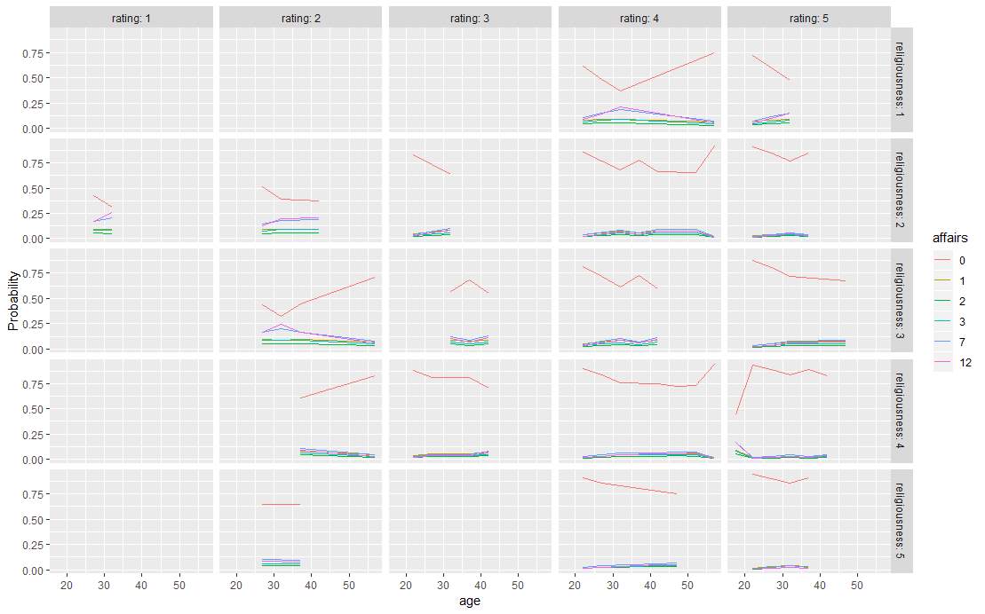
Figure 3 plots for all of the predicted probabilities for the different conditions.
From the plot, it is clear that the size of the test dataset is quite small, hence the plots for some conditions are incomplete. And since all predictors are categorical variable, the lines in the plot are broken lines. Though more evidence is needed before any definitive conclusion can be drawn, the benefits and shortcomings of using an ordinal logistic regression model to fit the “Affairs” dataset are discussed below.
The significant variables for the final ordinal logistic regression (OLR) model are the same as the quasi-Poisson and the negative binomial regression model –
(marital happiness),
and
(degree of religiosity). But the OLR can give the predicted probabilities of having different times of affairs for different observations exactly. Besides, as the response variable “affairs” is an ordinal data, OLR is a more proper method to fit the “Affairs” dataset better. However, there are also some limitations of treating the response variable as ordinal data:
- There are rather few statistical methods designed for ordinal variables.
- The parallel lines assumption in R system (which means that the intercepts are different for each category but the slopes are the same among categories) for OLR is rather difficult to test.
6 Conclusions and discussion
The primary purpose of this paper has been to develop a model to explain the relationship between the number of having affairs and other variables related to the demographic characteristics. The model frame for both count data regression and ordinal logistic regression, as well as their implementation in the R system for statistical computing, are reviewed. Incorporating the over-dispersion and excess zeros problems, hurdle and zero-inflated regression models is also considered for modelling. Moreover, the profits and limitations of treating the response variables as count data or ordinal data are discussed.
As a result, though the models applied are different, the coefficients for
(marital happiness),
and
(degree of religiosity) are always significant. Among several count data discussed in this report, the zero-inflated regression model can explain the data best. For the ordinal regression model, a set of plots for predicted probabilities for the different conditions are showed. Though more data are needed to obtain a more complete plot for each cell.
For the further task, it is meaningful to study on if the observations having affairs with the same person or not, their marital status after several years (which means that if cheating in the marriage would change the status of marriage), or even the parental influence to individuals. As the extent of having extramarital affairs is by no means small, this topic has reality content to research.
References
- Achim Zeileis, Christian Kleiber, Simon Jackman, 2008. Regression Models for Count Data in R. Journal of Statistical Software, 27(8).
-
Allison, P., 2012. When Can You Safely Ignore Multicollinearity?. [Online]
Available at: https://statisticalhorizons.com/multicollinearity - Bandini E, Fisher AD, Corona G, Ricca V, Monami M, Boddi V et al., 2010. Severe depressive symptoms and cardiovascular risk in subjects. J Sex Med, Issue 10, p. 3477–3486.
-
Bruin, J., 2006. newtest: command to compute new test. UCLA: Statistical Consulting Group.. [Online]
Available at: https://stats.idre.ucla.edu/r/faq/ologit-coefficients/ - Cameron; Trivedi, 1990. Regression-based tests for overdispersion in the Poisson model. Journal of Econometrics, 46(3), pp. 347-364.
- Chambers JM, Hastie TJ, 1992. Statistical Models in S. London: Chapman & Hall.
- D, L., 1992. Zero-inflated Poisson Regression, With an Application to Defects in Manufacturing. Technometrics, Band 34, pp. 1-14.
- Dobson, Annette J; Barnett, Adrian G, 2008. An Introduction to Generalized Linear Models. 3rd Hrsg. s.l.:CRC Press.
- Entry, I., 1990. Types of data: nominal, ordinal, interval, and ratio scales. Optometry and vision science, 67(2), pp. 155- 156.
- Fair, R. C., 1978. A Theory of Extramarital Affairs. Journal of Political Economy, 86(The University of Chicago), pp. 45-61.
- Fisher, AD; Corona, G; Bandini, E; Mannucci, E; Lotti, F; Boddi, V; Forti, G; Maggi, M, 2009. Psychobiological Correlates of Extramarital Affairs and Differences between Stable and Occasional Infidelity among Men with Sexual Dysfunctions. JOURNAL OF SEXUAL MEDICINE, 6(3), p. 10.
- Fisher, A. D., 2012. Stable extramarital affairs are breaking the heart. International journal of andrology, 35(1), p. 11.
- Fox, J; Monette, G, 1992. Generalized collinearity diagnostics. JASA, Issue 87, p. 178–183.
- Hilbe, J. M., 2014. Modeling count data. New York: Cambridge University.
-
Jackman, S., 2008. pscl: Classes and Methods for R Developed in the Political Science Computational Laboratory, Stanford University. R package version 0.95. [Online]
Available at: http://CRAN.R-project.org/package=pscl - Jay M. Ver Hoef, Peter L. Boveng, 2007. QUASI-POISSON VS. NEGATIVE BINOMIAL REGRESSION: HOW SHOULD WE MODEL OVERDISPERSED COUNT DATA?, Washington: Ecological Society of America.
- McCullagh, P., 1980. Regression models for ordinal data. Journal of the Royal Statistical Society, 42(2), pp. 109-142.
- Nelder JA, Wedderburn RWM, 1972. Generalized Linear Models. Journal of the Royal Statistics Society A, Band 135, pp. 370-384.
-
Philipp, J., 2019. Which variance inflation factor should I be using: GVIF or GVIF^(1/(2⋅df))?. [Online]
Available at: https://stats.stackexchange.com/questions/70679/which-variance-inflation-factor-should-i-be-using-textgvif-or-textgvif - Shirley Glass, Jean Coppock Staeheli, 2004. Not ‘Just Friends’: Rebuilding Trust and Recovering Your Sanity After Infidelity. New York: s.n.
-
S, J., 2008. pscl: Classes and Methods for R Developed in the Political Science Computational Laboratory, Stanford University. [Online]
Available at: http://CRAN.R-project.org/package=pscl - Venables WN, Ripley BD, 1997. Modern Applied Statistics with S-PLUS. 3rd Hrsg. New York: Springer-Verlag.
- Venables WN, Ripley BD, 2002. Modern Applied Statistics with S. 4th Hrsg. New York: Springer-Verlag.
- Vincent Calcagno, Claire de Mazancourt, 2010. glmulti: An R Package for Easy Automated Model Selection with (Generalized) Linear Models. Journal of Statistical Software, 34(12).
Cite This Work
To export a reference to this article please select a referencing stye below:
Related Services
View all


DMCA / Removal Request
If you are the original writer of this essay and no longer wish to have your work published on UKEssays.com then please click the following link to email our support team:
Request essay removal