Data Prediction Strategy for ROSSMANN
| ✅ Paper Type: Free Essay | ✅ Subject: Engineering |
| ✅ Wordcount: 1444 words | ✅ Published: 30 Aug 2017 |
Our task in this project is to predict 6 weeks daily sales for 1115 Rossmann stores located across Germany. Why is this important? This will help the stores maximize their profit by focusing on specific aspects to improve and help in inventory management to reduce operational costs.
Missing data in Rossmann was identified initially. After fine tuning the data, we did some statistical analysis on it to explore the depth of data and find the major elements which are changing our values. We made sure that our results are not biased. Analysis such as Principle Component Analysis and Correlation Analysis has helped us know, in detail, about the data elements which are important to consider when predicting sales. We have validated the conclusions our group made in the previous presentation (exploratory analysis) about the data through the results of statistics. Many other conclusions can be drawn by just looking at the analysis in the following sections of this report. Furthermore, we did linear regression to see the relation between customers and sales. As expected sales increased linearly with the increase in the number of customers. However, it performed poorly for other variables due to the non-linearity of the data.

In House Prices, there are a 79 factors over which we have to analyze the house prices. In order to first categorize the important factors influencing house prices, correlation analysis is done. Linear Regression and Step wise regression is also done to determine the important features for house prices in general, and in stepwise fashion. ANOVA was done for the neighborhood and house style to check whether the mean or individual house styles and neighborhoods was different or not. The standard hypothesis resulted false and it was displayed that individual neighborhoods and house-styles hold different average selling prices. The tests exhibited that 2.5 story houses were the priciest in house styles while 1 story houses were most popular. The NorthRidge neighborhood has the most expensive houses as per ANOVA, while North Ames comes out to be the most popular and one of the cheapest neighborhoods.
Data prediction strategy for ROSSMANN (for next phase):
To choose our prediction method for Rossmann we considered a number of factors. First being the size of the data. The Rossmann data is extremely dense with multiple variables. Second was which variables to use for prediction. For this we did a correlation analysis on minitab and found that customers, sales and promo were the most important hence we considered them. Third the data provides no customer information (just ids). Given the above factors we decided to use “gradient boosting” method for prediction (Jain, Menon, & Chandra, n.d.). Although our model improves on accuracy the main tradeoffs are reduced speed and user interpretability. We will ignore the values for the days when the stores are closed to refine the prediction.
Rossmann Data
Statistical Analysis Strategy:
Minitab was deployed to do statistical analysis such as Box Plot and Quantile Ranges, Histograms, Principle component analysis, Correlation analysis.
Matlab was used to do linear regression of Sales Vs Customers.
Statistical analysis was done to validate the hypothesis made in the Visualization Project and to explore the data in detail.
House Price Data:
Statistical Analysis Strategy:
Minitab was used to do statistical analysis such as Stepwise Linear Regression, Correlation analysis, Residual Plots and Value Plots
This report first covers the Rossmann Data exploration and then House Price exploration are presented.
MISSING DATA:
- Table 1 shows the values of head to head analysis of data sets given in Rossmann. As shown, Store data in Test sheet is not covering the range of stores covered in Train.
- There are 11 records which does not give any information of whether those stores are open or they are closed.
- Figure 1 shows that there are clearly less number of days registered in year 2014 after the 27th week. The reason for this is the missing values of 180 store IDs from 27th week to 52nd week of 2014.
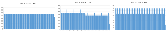
Figure 1. Year wise trend of Data Registered
Table 1 Head to Head Analysis of Data Sets
|
Number of Unique Values |
Unique Values |
NA Value Quantity |
||||
|
Field Name |
TRAIN |
TEST |
TRAIN |
TEST |
TRAIN |
TEST |
|
Store |
1115 |
856 |
– |
– |
||
|
Day of Week |
7 |
7 |
1,2,3,4,5,6,7 |
1,2,3,4,5,6,7 |
||
|
Date |
942 |
48 |
||||
|
Sales |
21734 |
– |
||||
|
Customers |
4086 |
– |
||||
|
Open |
2 |
2 |
1, 0 |
1, 0, NA |
11 |
|
|
Promo |
2 |
2 |
1,0 |
0 |
||
|
State Holiday |
5 |
2 |
0, a, b, c |
0, a |
||
|
School Holiday |
2 |
2 |
1,0 |
1,0 |
||
- Missing data set is assumed to be unrelated to actual values and may not be important. The data size is also smaller than the original data set, so ignoring the missing data will not lead to a biased result. Therefore, we considered missing data to be “missing at random” (Sazontyev & Lim, n.d.).
STATISTICAL ANALYSIS
Quartile Ranges
- Customers
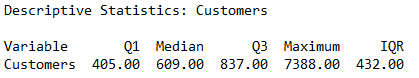
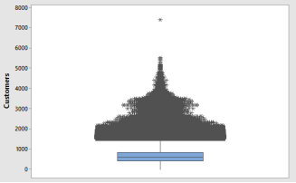
Figure 2. Box Plot of Customers
- Sales
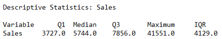
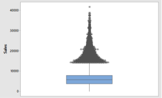
Figure 3. Box Plot of Sales
Histograms
Figure 4 and Figure 5 shows that our data is slightly right skewed. The frequency of customers and frequency of sales are higher when their values are low.
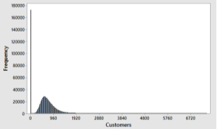
Figure 4. Histogram of Customers
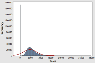
Figure 5. Histogram of Sales
Principle Component Analysis
Figure 6 shows the results of PCA in form of Scree Plot. We observe that the major effect on sales is due to customers (Component 1). Second influencing factor is the Number of stores which are open (Component 2). Promotions (Component 3) are influencing our sales but to a very low extent. We will also prove this via correlation analysis in coming sections.
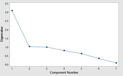
Figure 6. Scree plot of Train Data set
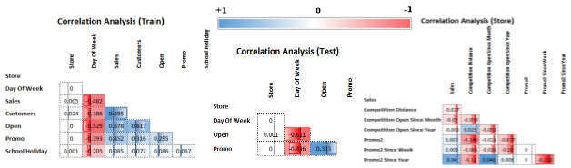
Correlation Analysis
Figure 7 shows the results of correlation analysis of the Rossmann Data. Cellular colors represent the intensity of correlations between the components. In the later sections, this correlation analysis is used to verify the results presented in visualization project.
Following are the prominent correlations:
Table 2 Major Correlation Results
|
Positive Correlated Components |
Correlation Value |
Negative Correlated Components |
Correlation Value |
|
Customers & Sales |
+0.895 |
Sales & Days of week |
-0.462 |
|
Store Open & Customers |
+0.617 |
Customers & Days of week |
-0.386 |
|
Store Open & Sales |
+0.678 |
Stores Open & Days of Week |
-0.529 |
|
Promo & Sales |
+0.452 |
Promo 2 & Competition Distance |
-0.146 |
|
Promo & Stores Open |
+0.295 |
Competition Distance & Sales |
-0.027 |
|
Sales & School Holidays |
+0.085 |
Promotions & School Holidays |
-0.067 |

 Correlation Matrices:
VERIFICATION OF VISUALIZATION RESULTS:
Claim 1: Sales decrease over the week.
Statistics Confirmation: This claim is verified through the correlation analysis. Correlation results of Sales Vs Day of Week is -0.462 (Table 2 and Figure 7). Which clearly shows the negative correlation between these entities.
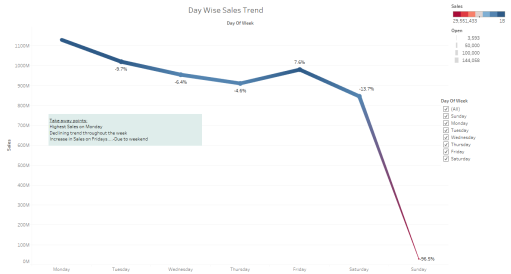
Figure 8. Day wise sales trend
Claim 2: Not much difference in sales when schools are open or close.
Claim 3: There are more Promotions when schools are open.
Statistical Confirmation: Correlation between Sales and School Holidays is +0.085 (Table 2 and Figure 7). As seen in Figure 9, sales when schools are closed is slightly greater than the sales when schools are open. This slight difference is proven by the small value of the correlation between these components.
Also, there are more promotions when schools are open (Figure 9). This is confirmed by the negative correlation of -0.067 (Table 2 and Figure 7) between promotions and school holidays.
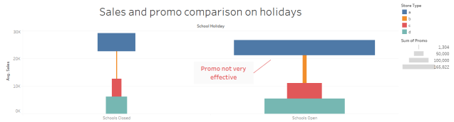
Figure 9. Sales and Promo Comparison on School Holidays
Claim 3: Sales increase with promotions but decreases with increase in competition distance.
Statistical Confirmation: Promotions and Sales are positively correlated by +0.452 (Table 2 and Figure 7). This positive correlation can be seen in the claim we made in last project (Figure 10). Orange peaks are the sales when the promotions are there. And mostly they are above the blue peaks. However, from Figure 10, we also observe that with increase in competition distance, our sales decreases. And this is validated by the negative correlation of -0.027 between sales and competition distance.
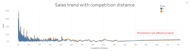
Figure 10. Sales Trend with Competition Distance
Linear Regression
Linear regression results in Figure 11 (obtained from Matlab) and Residual analysis results in Figure 12 (obtained from Minitab) show how sales is regressing with respect to the customers. The R2 value obtained is 0.8, which depicts that our linear regression is close to the data. Linear regression equation and regression coefficients is shown below:
B1 = 8.5238 ïƒ regression coefficient/slope
b1 = 1.077 and b2 = 0.0074 ïƒ Regression Equation (y = 1.077 + 0.0074x)
R2 = 0.8005
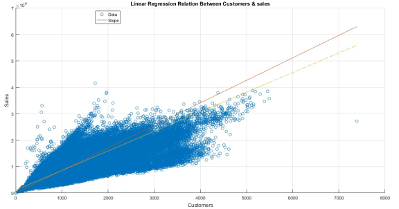
Figure 11. Linear Regression
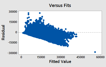
Figure 12. Residual Plot
STATISTICAL ANALYSIS
Regression Analysis
ï‚· Regression Equation
SalePrice = -323176 – 200.5 MSSubClass – 116.1 LotFrontage + 0.545 LotArea
+ 18697 OverallQual + 5227 OverallCond + 317.0 YearBuilt + 120.6 YearRemodAdd + 31.60 MasVnrArea + 17.39 BsmtFinSF1 + 8.36 BsmtFinSF2 + 5.01 BsmtUnfSF + 45.91 1stFlrSF + 46.68 2ndFlrSF + 34.2 LowQualFinSF + 8980 BsmtFullBath + 2490 BsmtHalfBath + 5390 FullBath – 1119 HalfBath – 10233 BedroomAbvGr – 21931 KitchenAbvGr + 5440 TotRmsAbvGrd + 4375 Fireplaces – 49.1 GarageYrBlt
+ 16788 GarageCars + 6.5 GarageArea + 21.5 WoodDeckSF – 2.3 OpenPorchSF
+ 7.2 EnclosedPorch + 34.6 3SsnPorch + 58.0 ScreenPorch – 61.3 PoolArea
– 3.85 MiscVal – 224 MoSold – 254 YrSold
ï‚· Regression Equation (STEPWISE)
SalePrice = -714877 – 202.0 MSSubClass – 106.7 LotFrontage + 0.545 LotArea
+ 18858 OverallQual + 6073 OverallCond + 326.0 YearBuilt + 31.29 MasVnrArea
+ 11.93 BsmtFinSF1 + 5.72 TotalBsmtSF + 46.77 GrLivArea + 9245 BsmtFullBath
+ 6171 FullBath – 10759 BedroomAbvGr – 22330 KitchenAbvGr
+ 5290 TotRmsAbvGrd + 4065 Fireplaces + 18107 GarageCars
+ 21.04 WoodDeckSF + 53.0 ScreenPorch – 59.7 PoolArea
Correlation Analysis
SalePrice MSSubClass LotFrontage LotArea OverallQual
MSSubClass -0.084
0.001
LotFrontage 0.352 -0.386
0.000 0.000
LotArea 0.264 -0.140 0.426
0.000 0.000 0.000
OverallQual 0.791 0.033 0.252 0.106
0.000 0.213 0.000 0.000
OverallCond -0.078 -0.059 -0.059 -0.006 -0.092
0.003 0.023 0.040 0.830 0.000
YearBuilt 0.523 0.028 0.123 0.014 0.572
0.000 0.288 0.000 0.587 0.000
YearRemodAdd 0.507 0.041 0.089 0.014 0.551
0.000 0.121 0.002 0.599 0.000
MasVnrArea 0.477 0.023 0.193 0.104 0.412
0.000 0.382 0.000 0.000 0.000
BsmtFinSF1 0.386 -0.070 0.234 0.214 0.240
0.000 0.008 0.000 0.000 0.000
BsmtFinSF2 -0.011 -0.066 0.050 0.111 -0.059
0.664 0.012 0.084 0.000 0.024
BsmtUnfSF 0.214 -0.141 0.133 -0.003 0.308
0.000 0.000 0.000 0.920 0.000
TotalBsmtSF 0.614 -0.239 0.392 0.261 0.538
0.000 0.000 0.000 0.000 0.000
1stFlrSF 0.606 -0.252 0.457 0.299 0.476
0.000 0.000 0.000 0.000 0.000
2ndFlrSF 0.319 0.308 0.080 0.051 0.295
0.000 0.000 0.005 0.051 0.000
LowQualFinSF -0.026 0.046 0.038 0.005 -0.030
0.328 0.076 0.183 0.855 0.245
GrLivArea 0.709 0.075 0.403 0.263 0.593
0.000 0.004 0.000 0.000 0.000
BsmtFullBath 0.227 0.003 0.101 0.158 0.111
0.000 0.894 0.000 0.000 0.000
BsmtHalfBath -0.017 -0.002 -0.007 0.048 -0.040
0.520 0.929 0.802 0.066 0.125
FullBath 0.561 0.132 0.199 0.126 0.551
0.000 0.000 0.000 0.000 0.000
HalfBath 0.284 0.177 0.054 0.014 0.273
0.000 0.000 0.064 0.586 0.000
BedroomAbvGr 0.168 -0.023 0.263 0.120 0.102
0.000 0.371 0.000 0.000 0.000
KitchenAbvGr -0.136 0.282 -0.006 -0.018 -0.184
0.000 0.000 0.834 0.497 0.000
TotRmsAbvGrd 0.534 0.040 0.352 0.190 0.427
0.000 0.123 0.000 0.000 0.000
Fireplaces 0.467 -0.046 0.267 0.271 0.397
0.000 0.082 0.000 0.000 0.000
GarageYrBlt 0.486 0.085 0.070 -0.025 0.548
0.000 0.002 0.018 0.355 0.000
GarageCars 0.640 -0.040 0.286 0.155 0.601
0.000 0.126 0.000 0.000 0.000
GarageArea 0.623 -0.099 0.345 0.180 0.562
0.000 0.000 0.000 0.000 0.000
WoodDeckSF 0.324 -0.013 0.089 0.172 0.239
0.000 0.631 0.002 0.000 0.000
OpenPorchSF 0.316 -0.006 0.152 0.085 0.309
0.000 0.816 0.000 0.001 0.000
EnclosedPorch -0.129 -0.012 0.011 -0.018 -0.114
0.000 0.646 0.711 0.484 0.000
3SsnPorch 0.045 -0.044 0.070 0.020 0.030
0.089 0.094 0.015 0.436 0.246
ScreenPorch 0.111 -0.026 0.041 0.043 0.065
0.000 0.320 0.152 0.099 0.013
PoolArea 0.092 0.008 0.206 0.078 0.065
0.000 0.752 0.000 0.003 0.013
MiscVal -0.021 -0.008 0.003 0.038 -0.031
0.418 0.769 0.907 0.146 0.230
MoSold&
Cite This Work
To export a reference to this article please select a referencing stye below:
Related Services
View all


DMCA / Removal Request
If you are the original writer of this essay and no longer wish to have your work published on UKEssays.com then please click the following link to email our support team:
Request essay removal